


- Ceramic tile surface defect detection with integrated feature engineering and defect fuse classifier
Chi Zhang*
Liaocheng Vocational and Technical College, Liaocheng, Shandong, 252000, China
This article is an open access article distributed under the terms of the Creative Commons Attribution Non-Commercial License (http://creativecommons.org/licenses/by-nc/4.0) which permits unrestricted non-commercial use, distribution, and reproduction in any medium, provided the original work is properly cited.
Introduction: Ceramic tile surface defect detection is crucial for ensuring product quality. This study proposes an integrated approach combining feature engineering and a Defect Fuse Classifier for accurate defect detection. Methods: The proposed model utilizes Python and splits the collected data into 70% for training and 30% for testing. Purpose: The purpose section explicitly states the objectives of the study. It highlights the research goals, such as evaluating the effectiveness of the proposed methodology in detecting ceramic tile surface defects and exploring the impact of parameter variations on detection performance. Results: Comparative analysis with state-of-the-art methods is conducted using various metrics such as sensitivity, specificity, accuracy, precision, FPR, FNR, NPV, F-Measure, and MCC. (a) For a Training Rate of 70%: The proposed Defect Fuse Classifier outperforms existing models with an accuracy of 97.4%, precision of 88.5%, sensitivity of 88.5%, specificity of 98.5%, F-Measure of 88.5%, MCC of 87%, NPV of 98.5%, FPR of 1.4%, and FNR of 11.4%. Conclusion: This study introduces a novel deep learning approach for ceramic tile surface defect detection, encompassing data acquisition, pre-processing, feature extraction, feature selection, and deep learning-based defect detection. The proposed Defect Fuse Classifier, integrating CNN, Bi-LSTM, and RNN, demonstrates superior performance, making it a promising solution for defect detection in ceramic tile surfaces.
Keywords: Ceramic tile, Defect detection, Hybrid optimization model, Defectfuse classifier.
Ceramic tile is a popular construction decoration, with mechanization and automation in manufacturing. The flaws like dirt, scratches, pinholes, uneven color, and corners can occur during the ceramic tile-making process [1]. High mechanical strength ceramic tile preparation reduces raw material consumption, manufacturing costs, waste emissions, and transportation costs, thereby improving the cost-performance ratio of goods [2]. Ceramic tile has chemical stability, design diversity, and stain resistance, but its high energy consumption and pollution emissions harm the environment despite its economic contributions [3]. Automated equipment is used for tile size and flatness checks, while manual labor is still used for surface quality examination, with defects detected through texture methods, with simple ones visible [4].
The industrial sector faces challenges in maintaining product quality in ceramic tile production, which is evaluated using automated visual assessment. Improving defect identification accuracy is a challenging task that can affect manufacturing quality, customer trust, and business earnings [5]. The ceramic tile industry utilizes quality control and defect detection at various manufacturing stages, often automated using computer vision and image processing techniques, enhancing efficiency and effectiveness [6]. Defects in ceramic tiles can be caused by unreliable manufacturing equipment, production procedures, and raw ingredients, resulting in physical harm, structural weaknesses, and cosmetic issues, affecting the tiles’ structural integrity and safety [7]. The technology develops an automatic visual inspection system that can detect surface fractures as thin as a hair’s width, evaluating its classification performance using network design optimization strategies and data augmentation methodologies [8]. Utilizing industrial cameras and image processing algorithms, machine vision inspection technology offers a novel method for identifying surface flaws in ceramic tiles [9].
Efficient quality control and performance of ceramic materials rely on non-destructive assessment techniques. The industry seeks automated computer-assisted inspection solutions to eliminate subjectivity and cost inefficiencies [10]. In the defect identification process, neural networks, specifically CNN, are commonly used. CNN is used to detect fractures and surface defects in raw images. Multiple CNN design algorithms exist, and developing the optimal CNN model for a specific task requires expertise and effort [11]. CNN-based target measurement algorithms have demonstrated impressive results in various industries. These algorithms have proven invaluable in the manufacturing industry’s quality control procedures, especially when it comes to measuring measurements and identifying product flaws. CNN-based target measurement algorithms have also been used in the aerospace sector to check for flaws and irregularities in aircraft components. These algorithms may discover surface flaws, fissures, and abnormalities that could jeopardize the aircraft’s structural integrity by analysing photos taken by inspection cameras or drones. Research has indicated that CNN-based algorithms exhibit higher sensitivity and dependability when compared to manual inspection methods or conventional image processing approaches.
The Faster Region-based convolution neural network (R-CNN) model employs the Soft-NMS method to detect flaws and combines multiple layers’ features. Faster R-CNN serves as a recognition framework with robust feature expression and easily modifiable structure [12].
According to the HSV color space, the defect discriminator was built using support vector machines (SVM) for two classes after the defects were separated using the conventional saliency detection approach. The color histogram characteristics for segmented defect rectangles were retrieved. At last, the algorithm produced the desired result of increasing fault detection accuracy [13]. The brightness histogram is widely used for identifying defects due to its simplicity and low complexity. The LBP offers improved accuracy but requires longer computation time compared to the luminance histogram [14]. A basic step in image analysis is edge detection, which includes locating the borders between various areas of a picture. A well-liked technique for edge identification in many applications is the Canny edge detection algorithm [15]. This paper aims to find the ceramic tile surface defect detection with integrated feature engineering and defectfuse classifiers.
The main contribution of this research work:
● To introduce a new optimization model: The proposed new hybrid optimization model for feature selection. The model used the Arithmetic optimization Algorithm and Dingo optimization respectively.
● To introduce a new defectfuse classifier model for surface defect detection: The considered defectfuse classifier model is the combination of CNN, Bi-LSTM, and RNN.
In 2020, Wang et al. [16] explored the increasing popularity of vision-based inspection methods in industrial manufacturing, focusing on surface flaw identification. It suggests a technique to minimize false positives that combines feature comparison analysis with adversarial and unsupervised learning.
In 2022, Nogay et al. [17] addressed the application of CNNs in deep machine learning to recognize ceramic flaws, highlighting the significance of both cost containment and product quality. It suggested using thermographic methods and contrasted 1D and 2D CNNs. Defect detection accuracy and resilience were significantly increased with DCNN models with transfer learning, according to a case study utilizing a pre-trained AlexNet-like model.
In 2022, Jinet al. [18] focused on developing a deep learning system for Automated Surface Defect Inspection (ASDI) in decorative ceramics. After preprocessing the images and training YOLOv3 on faulty images, they achieved a 94.90% detection accuracy at 25 frames per second. The decorative ceramics sector benefited economically from this algorithm’s increased inspection efficiency and quality.
In 2021, Sušacet al. [19] introduced a multi-line signal change detection method for identifying flaws in ceramic tile images, enhancing defect identification precision and effectiveness. It emphasized technology transfer for quality assurance in the ceramic tile sector, significantly contributing to image processing and flaw identification.
In 2021, Raiet al. [20] discussed the usage of deep learning for finding ceramic surface defects instead of laborious human examination. It examined deep learning techniques, with the greatest outcomes coming from ensemble learning. Customization and flexibility were provided via deep learning. The paper reviewed relevant literature with an emphasis on image-based manufacturing fault identification.
In 2023, Boovaneswariet al. [21] examined the application of AI’s deep neural networks are being used to identify defects in ceramic tiles, a shift from human inspection to image processing techniques. This involves addressing issues like form similarity and fabric classification, using various algorithms and techniques.
In 202, Qianet al. [22] explained that the framework automates the color-separation process for ceramic tiles, reducing human judgment. It uses HSV color space histogram statistics for preprocessing and feature extraction, training an SVM model, and balancing training time and accuracy.
In 2020, Leet al. [23] covered a learning-based method that makes use of tiny picture datasets to identify surface flaws. The authors suggested a technique for surface fault identification that made use of machine learning. The study brought attention to the difficulty of dealing with sparse data and offered a way around it.
In 2021, Junioret al. [24] discussed the importance of early detection of ceramic facade fractures in construction to ensure building integrity and passenger safety. Deep learning and image processing have improved crack identification systems, while image segmentation identifies fracture sites. Table 1 tells about the research gaps identified in the existing works.
Research Gap
Several authors have addressed the pressing research gaps in ceramic tile defect detection, each proposing distinct methodologies to tackle this challenge. Wang et al. (2020) aimed to develop an unsupervised technique for patterned texture surface images, filling the void in efficient defect detection without manual labeling. Nogay et al. (2022) targeted the detection of subtle deformations, addressing the delay in identifying faults in ceramic products, a gap often overlooked in defect detection systems. Jin et al. (2022) sought to automate decorative ceramic flaw inspection, addressing the need for sophisticated checks in this domain. Sušac et al. (2021) focused on signal change detection methods, a crucial area for enhancing efficiency in ceramic tile flaw detection processes. Rai et al. (2021) investigated deep learning techniques for industrial product surface problem detection, bridging the gap in efficient quality inspection methodologies. Boovaneswari et al. (2023) contributed to improving defect detection through deep neural networks, aiming to address the efficiency gap in quality control processes. Qian et al. (2021) proposed a color-separation framework based on the HSV color space and SVM model, addressing the need for advanced color-based defect detection techniques. Le et al. (2020) focused on learning-based defect identification, especially in scenarios with limited image datasets, filling a significant research gap in data-driven defect detection approaches. Junior et al. (2021) utilized deep learning and automated optical inspection to detect ceramic tile flaws more accurately, addressing the gap in advanced defect detection methodologies. These studies collectively contribute to advancing defect detection in the ceramic tile industry, addressing key research gaps and enhancing quality control processes.
The constraints noted in prior studies on ceramic tile fault identification are intended to be addressed by the suggested model. First off, our model provides a complete approach to defect detection by combining a variety of deep learning approaches, including CNN, Bi-LSTM, and RNN. This overcomes the drawbacks of individual methods as noted by Wang et al. (2020), Nogay et al. (2022), and Rai et al. (2021). Through this integration, the difficulties mentioned by Jin et al. (2022) and Sušac et al. (2021) are overcome and defects, including small deformations and patterned texture surface pictures, may be detected more accurately.
In addition, our model addresses the issues raised by Rai et al. (2021) and Le et al. (2020) about the availability of labeled data by employing sophisticated optimization techniques like ADOA and DOX for feature selection and fault classification. Through the utilization of these methods, our model is able to efficiently extract pertinent information from photos of ceramic tiles without requiring a great deal of human labeling, which improves defect detection procedures’ scalability and efficiency.
Additionally, as mentioned by Boovaneswari et al. (2023) and Junior et al. (2021), our model integrates a hybrid defect fusion classifier that combines the characteristics of different deep learning architectures, minimizing the constraints associated with individual approaches. This method boosts overall quality control effectiveness in the ceramic tile manufacturing sector and guarantees reliable fault identification in a variety of manufacturing scenarios. Overall, by fusing cutting-edge deep learning techniques with creative feature selection algorithms, our proposed model provides a comprehensive response to the difficulties in ceramic tile defect detection. This advances the state-of-the-art in quality control procedures for ceramic tile manufacturing and overcomes the limitations found in earlier research.
|
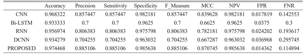
Table 1 Overall performance analysis for proposed Vs existing classifiers: for training rate=70% |
Overall Architecture
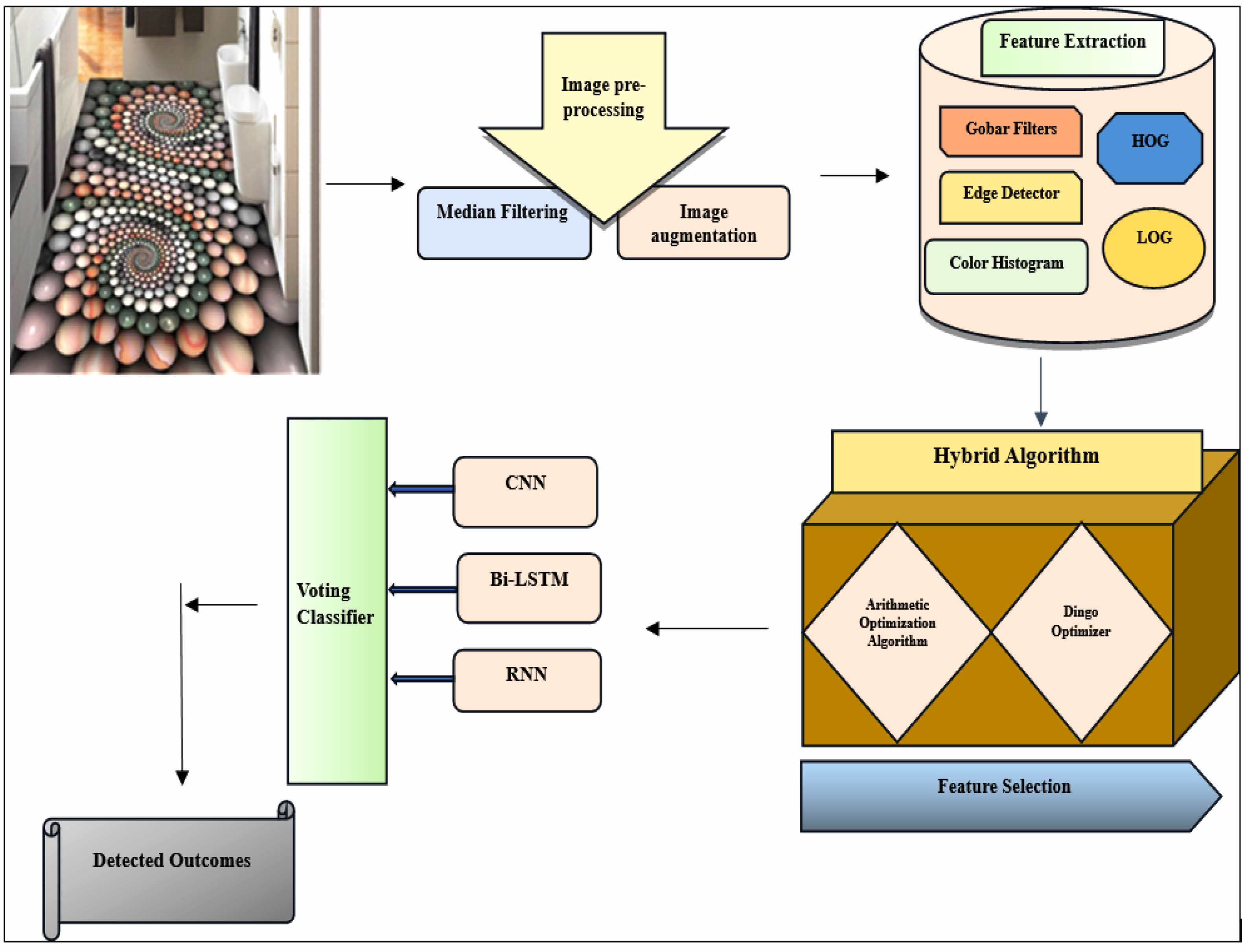
Defect detection in ceramic tile manufacturing is crucial for maintaining integrity, safety, and aesthetics. Machine Learning, trained on specific datasets, may not adapt to evolving defect types. Deep learning helps identify intricate patterns and minimizes the need for human feature engineering by learning and extracting features from images. Fig. 1 Fig. 2
In this research work, a new deep learning-based ceramic tile defect detection developed by the mentioned stages of the following: (i) Data Acquisition (ii) Image pre-processing (iii) Feature Extraction (iv) Feature Selection (v) Deep Learning based defect detection
Step 1: Data Acquisition
The dataset utilized in this investigation originates from the Alibaba Tianchi competition. The images are gathered by two separate lighting circumstances. In conclusion, a total of 4956 pictures were employed and saved in JPG format by the dimensions of 8192 × 6000 pixels. The dataset comprises six discrete classifications for defects observed on the external surface of ceramic tiles, namely, abnormalities in the borders, irregularities in the corners, imperfections resembling white dots, flaws in the light-colored blocks, flaws in the dark-colored blocks, and malfunctions in the openings.
Step 2: Image Pre-processing
The collected raw images are pre-processed via Median Filtering and Image Augmentation (rotation, flipping, brightness adjustments)
Step 3: Feature Extraction
From the pre-processed images, features like HOG, LBP, Color Histograms, Gabor Filters, and Edge Detector are extracted.
Step 4: Feature Selection
From the extracted features, the optimal features are selected using new hybrid optimization Algorithm. The Proposed hybrid optimization Algorithm is a combination for Arithmetic Optimization Algorithm and Dingo Optimizer, respectively.
Step 5: Deep Learning based defect detection
The defects in the tiles are identified via the new Defectfuse Classifier. This Defectfuse classifier is developed by combinin Deep Learning classifications like CNN, Bi-LSTM, and RNN, respectively. Finally, result from voting classifiers is validated.
Evaluation Metrics: The performance of the model is evaluated using various metrics such as accuracy, precision, recall, F1-score, and area under the receiver operating characteristic curve (AUC-ROC). These metrics provide insights into the model’s ability to correctly classify defective and non-defective tiles, as well as its trade-offs between false positives and false negatives.
Preprocessing
Preprocessing plays a crucial role in ceramic tile defect detection, and its importance can’t be overstated. It involves a series of image enhancement and cleaning techniques applied to raw images before defect detection algorithms are employed. Adjusting image contrast and brightness can make defects more visible. By enhancing the contrast between defects and the background, subtle defects that might be initially hard to spot become more apparent. Preprocessing techniques like edge detection help identify boundaries and edges within the image. Detecting edges can assist in segmenting the image and pinpointing defect locations.
In this research work the median filtering and image augmentation in pre-processing is done.
Median Filtering
Median filtering is the method employed in the realm of digital image processing to diminish noise and undesired variations while conserving crucial structural characteristics. It is particularly effective in removing “salt and pepper” noise, which is random, isolated pixels with extreme values [25]. The preprocessing method is highly regarded in surface defect detection, improving image quality and efficiency. It enhances image quality, making them suitable for visual scrutiny and automated identification of defect detection algorithms.
Steps to calculate Median Filtering
❖ A set of random variables is given. W = (W1, W2, ..... W0) The directive statistics are arbitrary variables. Considered by Ordering the Numbers of Wp in cooperative order. The median value is then expressed as per Eq. (1).
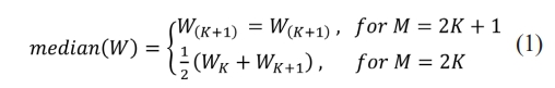
Where M = 2K+1 is the median rank. The median is utilized in an assortment of denoising and smoothing methodologies, particularly for signals that have been tainted by abrupt noise. It is acknowledged as a dependable evaluator of the positional element of a dispersion.
❖ The two-dimensional median filter for a grayscale input image with intensity values wi,l is defined as per Eq. (2).
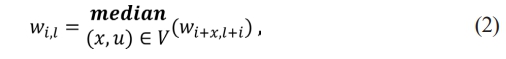
where V stands for the window that the filter can be used on. We examine M×M symmetric square windows with M = 2N+1, for the rest of the research, where M = (M 2+1)/2 is the median rank. Presumably, this is the filter version that is most frequently used.
❖ The median filter is useful for identifying specific image attributes by examining its output distribution and comparing it to other filters. However, its non-linear nature presents a significant challenge in theoretical investigations into the relationship between input and output distributions.
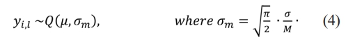
❖ Consequently, the widely recognized fact is that the input samples are indistinguishable. The typical Cumulative Distribution Function HY for productivity samples yi,l and source samples wi,l with Cumulative Distribution Function HW is provided as per the Eq. (3).
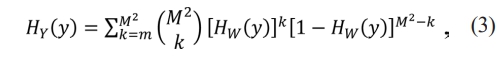
The sample median of input models with a standard dispersal is a unique yet fascinating example. 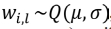 , which was displayed to asymptotically (as
  ) trail the standard distribution as per Eq. (4).
Typically, the combined arrangement of neighboring pixels has significance since close pixels in filtered images are slightly connected due to their overlapping windows. The M×M median filter with suggested input is HW(w). It generates an equation for both outcome pixels’ bivariate dispersion yr and ys (P), Hy(yr, ys). Even under the unrealistic premise that pixel intensities are in the case with Appendix (B) calculation, it is validated that defining median filtered images potentially poses challenges.
Image Augmentation
Image augmentation is extensively utilized technique in computer vision, machine learning, and deep learning. It artificially expands the dataset by applying different transformations to existing images. These changes may include cropping, rotating, flipping, adjusting brightness, and resizing, among other things. Tasks involving object identification, image segmentation, and image classification benefit greatly from image augmentation [26].
❖ Image augmentation allows you to artificially expand your dataset by generating additional images through various transformations. More data helps reduce overfitting in deep learning, where a large dataset is frequently associated with improved model performance.
❖ Augmentation enhances the utility of labeled data by generating additional examples without manual annotation, and it enables models to recognize defects with different characteristics and patterns, ensuring optimal surface problem detection.
❖ Augmentation improves surface defect detection models’ ability to identify new flaws beyond the initial training set, reducing overfitting, especially in small datasets. It enhances the model’s generalizability to new data, not just memorizing the training set.
3.3 Feature Extraction
The images from the pre-processing are extracted by the Feature extraction process. Feature extraction in ceramic tile defect detection involves capturing and representing essential characteristics from the input images to enable effective analysis and classification. Detecting surface defects frequently requires manipulating high-dimensional data, including images. Excessive dimensionality raises the possibility of overfitting and increases computational complexity. Feature extraction is important in ceramic tile surface defect detection process.
In this work, features such as HOG, LBP, Color Histogram, Gabor Filters, and Edge Detectors are extracted from the pre-processed images.
3.3.1 Histogram Of Oriented Gradient (HOG)
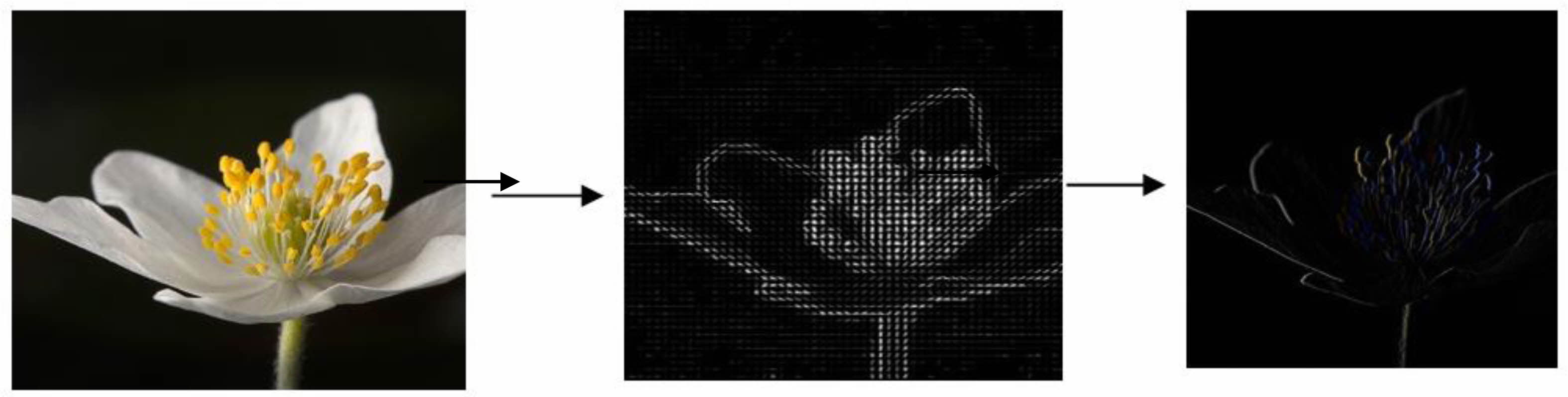
HOG is the feature extraction technique used in computer vision and image processing. It serves a multitude of purposes, encompassing object detection and image classification. The utility of HOG is especially evident in its ability to detect and identify objects or patterns within images [27]. HOG offers a cost-effective method for detecting ceramic tile defects, helping localize their positions within images. It’s effective in detecting edges and gradients, identifying fine edges and abrupt changes in the tile’s surface, which may indicate defects like cracks, chips, or surface irregularities. This information is crucial for quality control and repair.
Steps to calculate HOG Features
❖ Select the input image (pre-processed image) whose HOG characteristics need to be computed. 128 by 64 pixels, or 128 pixels in height by 64 pixels in width, is the required scale for the images. Enhancing performance on the site safety detection test was the main goal of employing this type of identification.
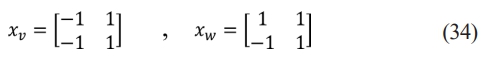
❖ The gradients of the image must be calculated before the HOG feature can be computed. A directed shift in pixel intensity along the v-axis and w-axis is known as an image gradient. The gradient vector of pixels at point (v, w) represents as per the Eq. (5)
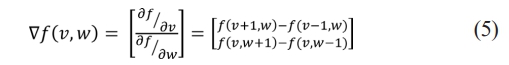
Where f (v, w) is the pixel intensity at coordinates v and w; hv and hw are the gradient in v and w direction, respectively. The magnitude, n(v, w) and phase, q(v, w) of the gradient, then can be calculated using the following Eq. (6) and Eq. (7), respectively.
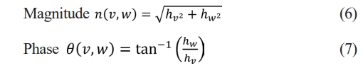
Where hv and hw are the gradient in v and w direction, respectively
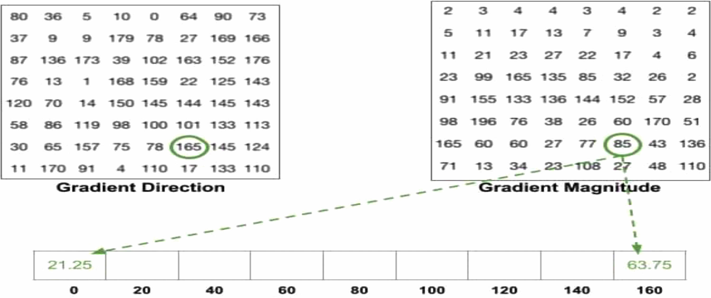
The gradient matrices are divided into 8×8 cells to form a block once the gradient of each pixel is determined. Each block is then used to compute a nine-point histogram. A nine-point histogram consists of nine bins, each representing a range of angles of twenty degrees. In Fig. 3, a nine-bin histogram is shown with values assigned based on computations. Each of these histograms might be represented as histogram with bins corresponding to angle intensity in the bin.
There are 64 distinct values in a block, so the computation is done for each of these values.
Number of bins = 9(starting from 0o to 180o)
step size (Dq) = 180o/Number of bins = 20o
Each Lth bin, Bin is separated as per the Eq. (8):
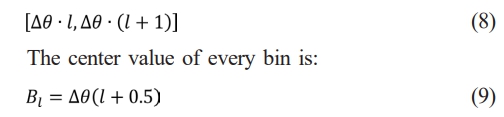
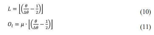
The lth bin and the value supplied to the lth and (l + 1)th bins is computed for every cell in the block. The value is determined using as per Eq. (10), Eq. (11), Eq. (12).
❖ A block’s bin is an array, to which the values of Ol and Ol+1 are attached at index for kth and (l +1) bin, respectively, determined for every pixel.
❖ The resultant matrix, as indicated by the computations above, is 16×8×9.
❖ The 9-point histogram matrix was combined into a new block (2×2), and the overlapping clubbing with an 8-pixel stride was performed, resulting in a 36-feature vector. Fig. 4. shows the method for calculating 9-bin histograms.

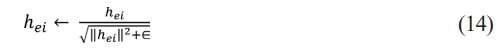
❖ The K2 norm is employed to standardize the standards of fb for each block:
❖ Before normalizing, the value l is first calculated through the subsequent Eq. (15), Eq. (16).
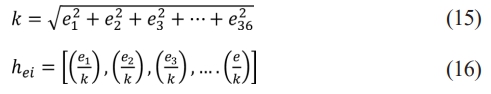
❖ The normalization process reduces contrast discrepancies in images of the same object by normalizing each brick in sequence. A feature vector is created by accumulating 36 data points, 15 blocks in a vertical direction and 7 blocks in a horizontal direction. The cumulative length for HOG features is calculated to be 3780.
Local Binary Patterns (LBP)
LBP is texture descriptor employed in computer vision and image analysis. When analyzing a pixel’s surrounding neighborhood, LBP takes into account the local patterns of pixel intensities in that area [28]. LBP is highly effective in describing and capturing local texture patterns in images. It is especially helpful in applications like texture segmentation and classification where texture information is essential. It generates histograms of the frequency of different local patterns, providing a concise representation of the texture distribution in an image or region.
Steps to Calculate LBP Features
❖ LBP is a technique that can analyze local textures in ceramic tile images, detecting variations that may indicate defects and can be used to extract texture features.
❖ The integration of LBP and deep learning in identifying defects on ceramic tile surfaces can improve detection accuracy by recognizing texture patterns, enhancing generalization, and providing a more reliable method.
❖ The combination of handcrafted features like LBP with deep learning techniques leverages the strengths of both approaches for more effective defect detection.
Assume that Ie = I(V, W) is an arbitrary central pixel at the position (V, W) and It = I(Vt, Wt) is a neighboring pixel surrounding Ie, with as per the Eq. (17), Eq. (18).
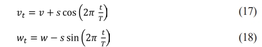
T is the total number of neighboring pixels (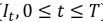 ) and S is the distance from Ie at which the pixels are sampled. The traditional LBP descriptor as per the following Eq. (18), Eq. (19)
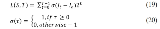
Where Ie denotes gray value of centre pixel. It denotes gray value of its neighbors. S stands for number of neighbor and T be the radius of neighborhood.
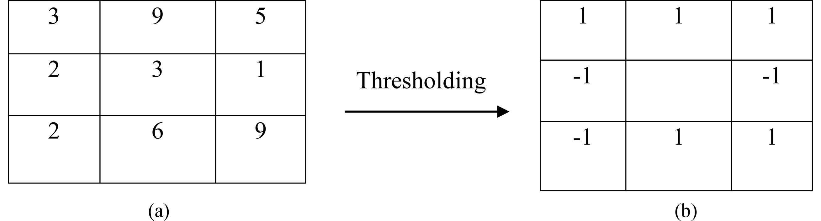
The actual 3×3 construction is shown in both Fig. 5(a) and 5(b). The structure in the figure has vectors of “[3,1,5,9,3,2,2,6,9]”. The sign vector in figure is “[-
1,1,1,1,-1,-1,1,1]”. It apparent that the novel regional binary pattern, which codes the binary digit as the 8-bit string “01110011” uses only the sign vector
❖ The LBPS,T operator generates (2T ) output values, forming dissimilar binary patterns by T pixels in neighbor set. Rotation effects are eliminated by assigning unique identifiers. The image rotates, causing gray It to move circle perimeter, Ie eliminate the rotation effect, and a unique identifier is assigned to each rotation using invariant local binary patterns. as per Eq. (21).

Where ri means rotation constant. ROR (v, b) be a rou nd bitwise turn right on T-bit number v, b times. Finally, the lowest of computed values ofb=0 to t-1 are chosen.
Color Histogram
A color histogram is a visual representation of color distribution within an image, providing a numerical assessment of each color’s quantity. It is created using the image’s color channels, where each channel’s histogram represents the intensity distribution for its corresponding color [29]. These are highly efficient feature vectors can be used in various image processing tasks, including object identification, content retrieval, and flaw identification, by condensing the color composition of an image.
Steps to Calculate Color Histogram Feature
❖ Color histograms can be effectively used in ceramic tile defect detection to analyze and characterize the color distribution within tile images. It can inform the setting of adaptive thresholds for defect detection.
❖ Adaptive thresholding techniques based on the color distribution can dynamically adjust the sensitivity of the defect detection algorithm.
❖ The RGB color space has three color component values. In our method, we utilized the HSV color space which aligns with the human visual system.
○ The HSV color space is used to extract color information from ceramic tile photos for defect detection in the context of the defect discriminator. The defect discriminator makes use of the hue, saturation, and value components of the picture pixels to detect minute color changes that might be signs of defects such surface imperfections, fissures, or discolorations.
○ The hue component can be used by the flaw discriminator to separate particular colors linked to defects, such dark patches or discolored areas. The value component provides information about the defect’s brightness or contrast in relation to the surrounding areas, while the saturation component can aid in determining how intense these colors are.
○ The defect discriminator can efficiently discern between normal and faulty regions in ceramic tile photographs by evaluating these color properties in the HSV color space. This allows for precise and efficient defect identification in production processes.
❖ RGB image changed into HSV color space as per the Eq. (22), Eq. (23), Eq. (24) respectively. (Here R is represented as S, G is represented as H and B is represented as A)
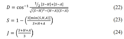
The color space values in an image are represented by the wavelength (D), saturation (S), and the intensity value (J). range from 0 to 1, representing the intensity of an image, with 0 representing black and 1 representing white.
❖ A set of bins representing individual colors in the color space being utilized is color histogram. The quantity of colors in the image determines the number of bins. A vector is what defines a color histogram as per the Eq. (25).

Where p denotes the color bin within the color histogram and D[p] denotes the count for pixels with color p in image, while n signifies total count of bins utilized in color histogram. Every pixel in image is allocated to bin in the color histogram based on its color. The value for each bin represents count of pixels with similar color. The normalized color histogram, denoted as D, is defined as per the Eq. (26).
Where 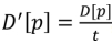 , t is total number of pixels of images
However, the color histogram has limitations of its own. The right photos cannot be retrieved if two images have the same color percentage but differ in how the colors are dispersed. Fig. 6. shows two unconnected images that have the same color histogram.
We extract the color histogram of the image and we get a n-dimensional color feature vector:
Histogram intersection method is used to measure the distance X1 between query image R and image T in image database.
Gabor Filter
Gabor filters are used to analyze and characterize textures in images, identifying patterns like edges, lines, and regions with specific textures. They are effective in identifying edges and curves, and their reaction to texture and intensity changes is noticeable [30]. They are particularly useful for capturing and analyzing textures on ceramic tile surfaces, enhancing textural patterns indicative of defects.The images serve as a feature representation that highlights relevant information about the texture and structure of the ceramic tile surface. These features can be fed into machine learning models for defect classification.
Steps to calculate Gabour Filter
(1) Gabour image generation
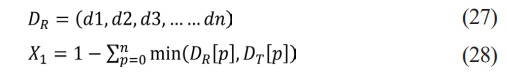
The following equation, which shows eight amplitudes (la) and eight phases (qb), respectively, yields a total of 64 Gabor filter as per the Eq. (29). Each Gabor filter measures 3×3.
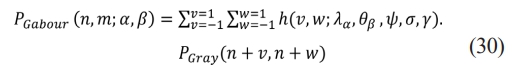
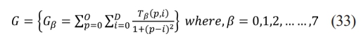
A picture with a gabor filter PGabour. The Gabor filter and the IGray are constructed by convolutionally operating on the former as per the Eq. (30).
(2) Steps for Gabour Image Selection
The images that have the lowest Inverse Difference Moment (IDM) value, N are chosen. The image with a significant variation in values between pixels is said to have a small IDM. With the chosen Gabor Image, efficient feature extraction for detection is achievable. The subsequent steps are in the Gabor image selection method.
Step 1: For each phase, construct average image P'Gabour for the Gabor image as per the Eq. (31).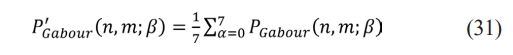
Step 2: The image of the Gabor filter is normalized P'Gabour as per the Eq. (32).
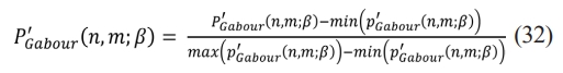
Step 3: According to the above equations the Gabor filter image P'Gabour (n,m;β) becomes a GLCM, from which the average matrix Tb is derived.
Step 4: Values for IDM features are taken out of each average matrix Tb as per the Eq. (33).
Step 5: The highest IDM feature values among the top M Gabor filter images are chosen.
Edge Detectors
An edge detector is an essential part of computer vision as well as the processing of images that locates areas in an image where there are noticeable changes in color or brightness. Edges often correspond to boundaries between objects or changes in texture, and detecting them is fundamental for various tasks, including object recognition, image segmentation, and feature extraction [31]. Understanding the composition and substance of images begins with edge detection. The Canny edge detector can be employed in ceramic tile surface defect detection for various purposes, contributing to the identification and characterization of defects.
Steps to calculate Edge Detectors
❖ The detected edges can be utilized as cues for segmenting and isolating defective regions on ceramic tiles. It helps in defining the contours of defects, facilitating the creation of regions of interest for subsequent analysis.
❖ Canny edges serve as features that capture the discontinuities and transitions in intensity on ceramic surfaces. Machine learning models that categorize and describe various fault kinds may be trained using extracted edge characteristics as input.
❖ Gaussian filtration is used to smooth the gradient’s direction and amplitude in the images. The gradient’s magnitude and direction are found using the finite difference method of the first-order partial derivative, as per Eq. (34), Eq. (35), Eq. (36), Eq. (37), Eq. (38) respectively.
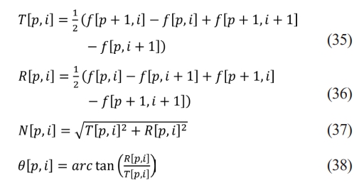
Here, the variable f represents gray value of image. The symbol T is used to denote the gradient amplitude in the V direction, while R represents the gradient amplitude in the W direction. The variable N is defined as the amplitude of the point under consideration. Lastly, the symbol q corresponds to the gradient direction, specifically the angle at which it is measured.
Feature Selection
The models from the extraction are selected in the feature selection process. Feature selection is a relevant attribute improves machine learning models by enhancing efficiency, preventing overfitting, and aiding interpretability. In deep learning, neural networks automatically learn features, and techniques such as regularization, attention mechanisms, and ensemble methods contribute to implicit feature selection. The features are selected via ADOA (Arithmetic Dingo Optimization Algorithm).
The significance of the newly developed hybrid optimization model for feature selection is noteworthy when it comes to the identification of surface defects in ceramic tile, and it may also find use in other fields. Here are some main justifications for its significance:
● Enhanced Performance of the Model: This integration of AOA and DOA, makes it possible to search for ideal characteristics more thoroughly and effectively, which improves the model’s performance in defect identification.
● Effective Feature Selection: Finding the most pertinent characteristics while lowering dimensionality is made possible by feature selection, which is a crucial stage in the creation of machine learning models. By effectively navigating the feature space and choosing the most discriminative features for defect detection, the hybrid optimization model maximizes the feature selection procedure.
● Adaptability to Data Characteristics: The hybrid optimization model’s adaptive nature enables it to dynamically modify its methods in response to the properties of the incoming data. This flexibility is especially important for defect identification, as different types and patterns of flaws may occur, and it guarantees that the model can handle a wide range of circumstances.
Overall, the proposed hybrid optimization model for feature selection plays a crucial role in improving the efficiency, effectiveness, and interpretability of defect detection models, thereby contributing to higher product quality and operational efficiency in industries such as ceramic tile manufacturing.
Arithmetic Optimization Algorithm
Arithmetic Optimization Algorithms improve numerical computation efficiency and accuracy by optimizing precision, minimizing errors, and improving mathematical performance. They address challenges in floating-point arithmetic, reduce complexity, and explore parallel computing for faster execution [32]. Adaptive approaches dynamically adjust algorithms based on input characteristics, crucial in scientific computing, machine learning, and numerical simulations.
Population-based algorithms use random solutions, while detection-based algorithms use randomization for optimal solutions. Optimization involves exploration and exploitation, with exploration preventing local solutions and exploitation improving the precision of answers during the investigation phase.
Initialization phase
The collection of candidate solutions for AOA is chosen randomly and starts the optimization process (W), as indicated in matrix Eq. (39).
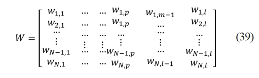
Before commencing work, the AOA ought to determine which search phase exploration or exploitation. The following search phrases employ the Math Optimizer Accelerated (MOA) function, whose factor was obtained using as per the Eq. (40).
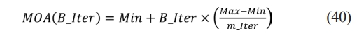
MOA(B_Iter) is the function value at the Cthiteration, as identified as per Eq. (40). B_Iter defines current iteration between 1 and greatest number of iterations (m_Iter). The characters Min and Max, respectively, refer to minimum and maximum values of accelerated function.
Exploration phase
The AOA explores using the division (d) and multiplication (m) operators, which have scattered values and cannot easily approach the objective. By using four mathematical operations, the exploration search finds the nearly ideal solution. The operators (d and m) assist with the exploitation step of the search process.
The exploration stage of the AOA involves randomly investigating the search area using the division (d) and multiplication (m) operators. The Math Optimizer Accelerated (MOA) function guides this process based on a random number. The first operator (d) is activated when t2 < 0.5, and it performs its task until completed. During this time, the second operator (m) remains idle. If t2 >= 0.5, the second operator (m) takes over the current task rather than d. The operators are activated based on specific conditions and promote diversification and exploration through a stochastic scaling coefficient. The exploration phase in AOA efficiently searches for better solutions while promoting exploration and diversification. The position-updating equations are proposed to facilitate the process as per the Eq. (41).
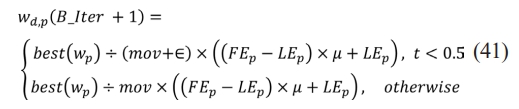
where wd,p(B_Iter) indicates the pth position in the dth solution in the current iteration, wd,p(B_Iter + 1) indicates the dth solution in the following iteration, and best(wp) represents the pth place in the best solution thus far, KCi and ACi represent upper and lower limit values of pth slot, respectively, while e is a small integer. The search process is controlled by m, which has a fixed value of 0.5 based on the tests reported in this work as per the Eq. (42).
Where (m_Iter) is extreme number of iterations, (mop) is coefficient, and function value at uth iteration indicates mop (B_Iter) signifies the current iteration. The work’s experiments indicate that the exploitation accuracy across repetitions, denoted by the sensitivity limit a, is set at 5.
Exploitation phase
The AOA employs an exploitation approach based on mathematical computations using Subtraction (s) or Addition (a) operators. These operators have low dispersion characteristics and are proficient at detecting near-optimal solutions. The exploitation phase utilizes these operators to facilitate enhanced communication and support within the optimization process.
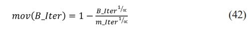
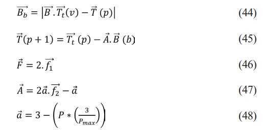
The initialization of this stage is determined by the MOA function value, with specific requirements outlined. The exploitation operators thoroughly examine dense regions in the search area to approach and discover enhanced solutions based on two primary search strategies. These strategies are effectively represented as per the Eq. (43).
Deep search is used to explore the search space, employing two main operators, s and a, to exploit the space. The first operator s is activated based on a condition, while the second operator a remains inactive. If t3 is less than 0.5 a takes over. These procedures resemble the partitioning approach but are designed to avoid getting stuck in local areas, ensuring optimal solutions and maintaining solution diversity. Stochastic values are generated to ensure exploration throughout iterations.
The final position in a search can be stochastic, estimating the near-optimal solution, while other solutions update their positions around this solution.
Dingo Optimization Algorithm
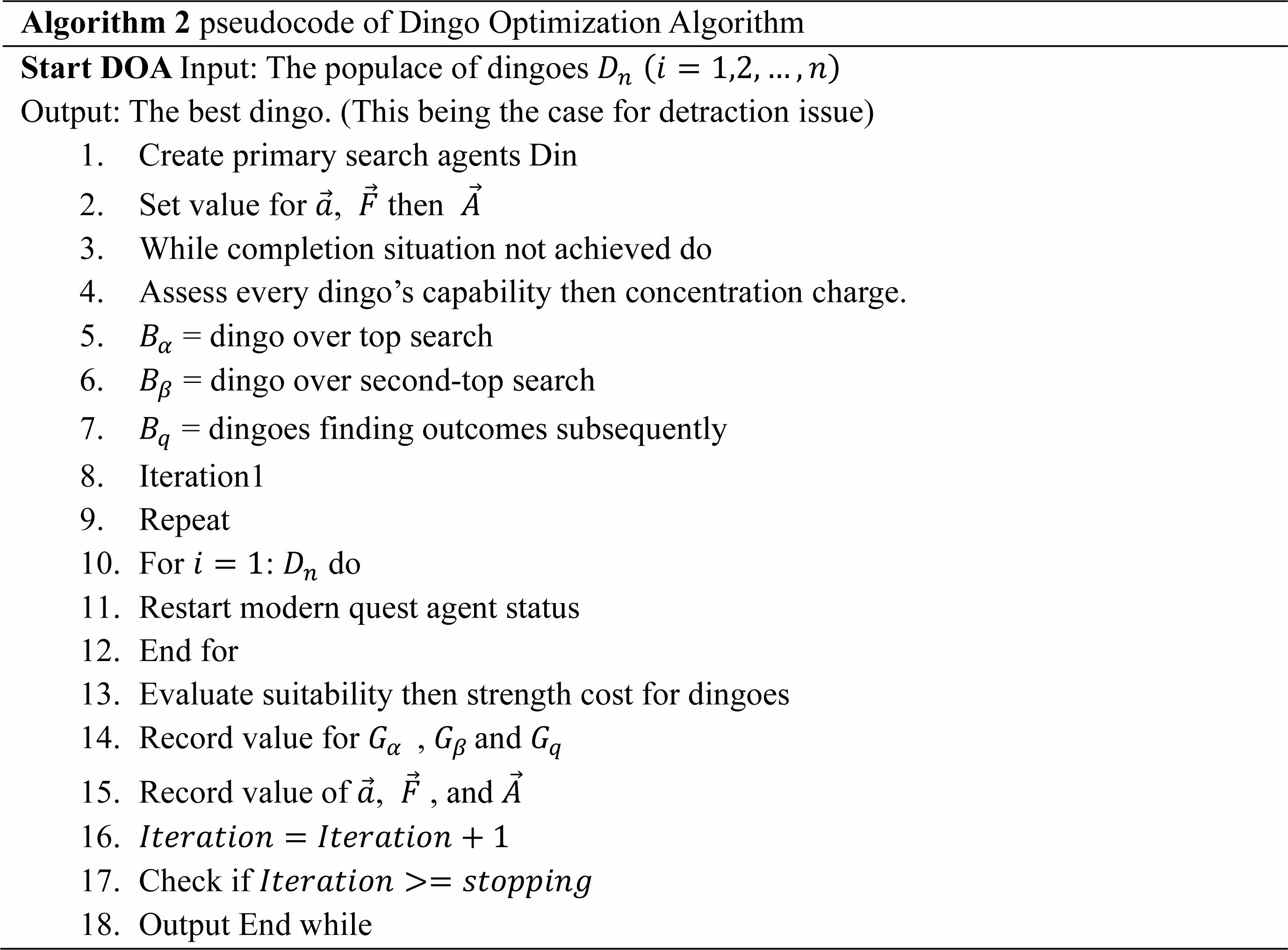
The Dingo Optimization Algorithm mimics the behavior of dingoes to solve optimization problems. It employs a population-based approach. Dingoes collaborate to find the optimal solution through exploration and exploitation of solution space. Each dingo represents a potential solution, also the algorithm evolves the population by adapting to the fittest solutions. The Dingo Optimization Algorithm is effective in diverse fields such as engineering, machine learning, and logistics, as it harnesses principles from the natural behavior of dingoes.
Mathematical Models
Dingo optimization is carried out in this part by the mathematical design of the model of the hunting, surrounding, and attacking prey.
Encircling
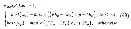
Dingoes are intelligent and locate their prey, surrounded by pack and alpha. The social hierarchy of dingos suggests the objective prey represents the best agent strategy, as the search region is unknown. Other search companies are updating their plans for potential strategies. The dingoes’ behavior is patterned as per the Eq. (44), Eq. (45), Eq. (46), Eq. (47), Eq. (48).
Where  is distance among dingo and prey.
  be position vector (prey).
  be the position vector (dingo).
  and
and  be a Coefficient vector.
  and
and  be the Random vector in [0,1].
  be a Linear reduction from 3 to 0 at all iterations. P be 1, 2, 3, ……, Pmax. Pmax be Maximum no. of iteration.
Hunting
Dingoes are unaware of the optimal prey location in their search area. However, alpha, beta, and other dingos know the potential location and can mimic hunting behavior. Alpha usually leads hunting, but beta or other dingos may also hunt. Two best values are considered to determine the optimal position for the prey. To do this, all dingoes must update their locations, which may be expressed mathematically as per the Eq. (49), Eq. (50), Eq. (51), Eq. (52), Eq. (53), Eq. (54).
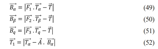
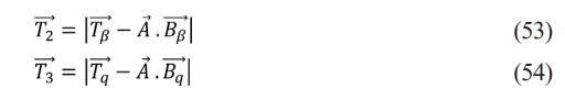
To calculate intensity of every dingo, following as per the Eq. (55), Eq. (56), and Eq. (57) are being used,
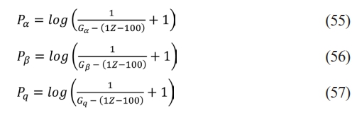
where, Ga and Gb = a and b-dingo fitness values, correspondingly, Gq = another dingo fitness worth.
Attacking Prey
Dingo completes hunt by attacking if no position update. Approach is mathematically constructed by lowering value of  . The range
  is decreased by ,
  variable
  within an [-3a, 3a] interval is randomized, a value is decreased, when a variable has random values between [1, 1], the next position could be anywhere between current and preys.
Searching
Dingoes hunt according to the group’s position. The DOX uses random values,  , to scan targets worldwide, indicating approaching or running prey. A value greater than 1 indicates approaching prey, while a value less than -1 indicates running prey. also increases exploration possibilities. The vector
  in Eq. (46) can generate any random number between [0, 3] for varied prey weights. The variable DOX is a probabilistic variable, where vector ≤ 1 comes before vector ≥ 1 for analyze impact of the gap as stated in Eq. (44).
ADOA
In ADOA, the mean of the acquired best solution from AOA and DOX is computed. This means the computed best solution is the global best solution.
Advantages:
● The best solution will be efficient and a positive impact on defect detection.
● The best solution will find the defect fastly and accurately.
● It enhances workflow, enabling both teams and individuals to work more and provide better job outcomes.
The mean is for the utilization of the best solution in both algorithm
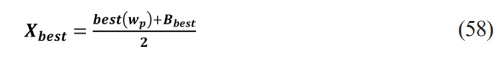
Xbest, be the overall global best solution. best(wp)be the best solution (in terms of position) acquired from AOA. Bbest be the best solution (in terms of position) acquired from DOX. Mathematically, ADOA algorithm can be given as per Eq. (58).
DefectFuse Classifier
The selection feature next comes to the defectfuse classifiers. The defectfuse classifiers is the combination of CNN, Bi-LSTM, RNN, and Voting classifier.
CNN
CNN are Strong deep learning models were developed particularly for applications related to computer vision and image processing. CNNs consist of pooling, fully connected, and complexity layers. These layers automatically extract layers of information from input images [33]. CNNs’ capacity to capture spatial hierarchies and patterns makes them useful for applications like item identification, facial recognition, and image classification. CNNs are ANNs (artificial neural networks) extended to feature extraction from matrix datasets with grid-like structures. Shared-parameter neural networks are called CNNs. Consider a representation of image as a cuboid whose length, width, and height are the RGB channels and image’s dimensions.
In a CNN model, the input x of every layer is arranged in three dimensions: height, width, and depth, or n×n×s, where n is similar as the width. Another name for the depth is the channel number. For instance, the depth (r) of an RGB picture is three. There are several kernels, or filters, denoted by l in each convolutional layer. Similar to the input image, they contain three dimensions (m×m×r); the only requirements are that m must be smaller than n and that q must either be equal to or smaller than s.
Furthermore, the kernels serve as the foundation for the local connections, which, as was previously indicated, convolve with input and share identical characteristics (weight Oι and bias αι) for producing ι feature maps αι with a size of (n-m-1) each f is the activation function applied element-wise v represents input data * represents the convolution operation. The inputs are small portions for original picture size, and convolution layer computes dot product among its input and weights as in Eq. (59).
Bi-LSTM
Bi-LSTM, is pattern model has two LSTM layers: one to process inputs in the direction of progress and another for handling in the reverse direction. It is typically applied to jobs using NLP. The idea behind this strategy is that the model can better comprehend the link between sequences by processing input in both directions.
The gradient of a recurrent neural network can quickly inflate also vanish in the gradient method when the time steps are excessively little or big. Consequently, LSTM utilizes a gating mechanism to regulate information to tackle this difficulty. The hidden state among earlier time step Du-1 and the present time step input Vu is the input of an LSTM gate. The entire connecting layer calculates the output as per the Eq. (60), Eq. (61), Eq. (62), Eq. (63), Eq. (64).
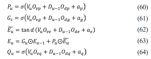
d signifies the number of secret units, Vu means the tiny batch input over the time step p, Du-1 denotes the secret state for preceding time step, s represents the sigmoid function, Ovp and Odp denote the weight matrix for gate used for input, also ap is the input gate’s offset term. Ovg and Odg represent weight matrices for forgetting gate, and ag is forgetting gate’s offset term. As potential memory cells, Eu represents the current cell state, Eu-1 represents the prior cell state, Ove and Ode are weight matrices of gated unit, and ae is offset term for gated unit. Ovq and Odq are weight matrix for output gate, then aq is the offset term for output gate. The concealed state’s information flow is regulated by multiplication by elements .
Data flow from memory cell to hidden state is regulated by output gate Qu, and the resultant output Du as per the Eq. (65).

The Bi-LSTM technique uses both forward and reverse LSTM to extract features from data, considering all hidden details. This method can improve the results by merging two-way extraction results from two dimensions in a specific method, reducing the data provided by single LSTM and resulting in more comprehensive results.
RNN
An artificial neural network class called RNN is made for processing data sequentially. Because of their special design, they may be used for tasks like time series prediction, voice recognition, and language modeling, and they can retain hidden states that reflect temporal relationships. RNNs preserve the recollection of previously processed data as they step-by-step process incoming sequences. However, the problem of vanishing gradients is the reason behind its incapacity to express long-term dependency.
The Gated Recurrent Unit (GRU) is popular RNN unit that can capture relationships over various time scales adaptively. It features gating units that influence stream of detail, similar to LSTM units. However, GRU exposes the entire state every time and lacks regulation mechanism. Due to the disparity in length between questions and answers in AS, it is more suitable. To learn sentence representations, the hidden state du is calculated as per the Eq. (66), Eq. (67), Eq. (68), Eq. (69).
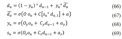
where O, Oy, Os; C, Cy, Cs and a, ay, as are network parameters.
Voting Classifiers
Voting classifiers in deep learning are used to detect defects by integrating the outputs of several different models to determine whether or not a flaw exists. This ensemble approach improves accuracy and resilience by using many models [34]. Voting classifiers are essential to obtaining high accuracy and resilient performance in defect detection applications because they use the advantages of many deep learning architectures to make collective choices regarding the existence of faults in a variety of materials or surfaces.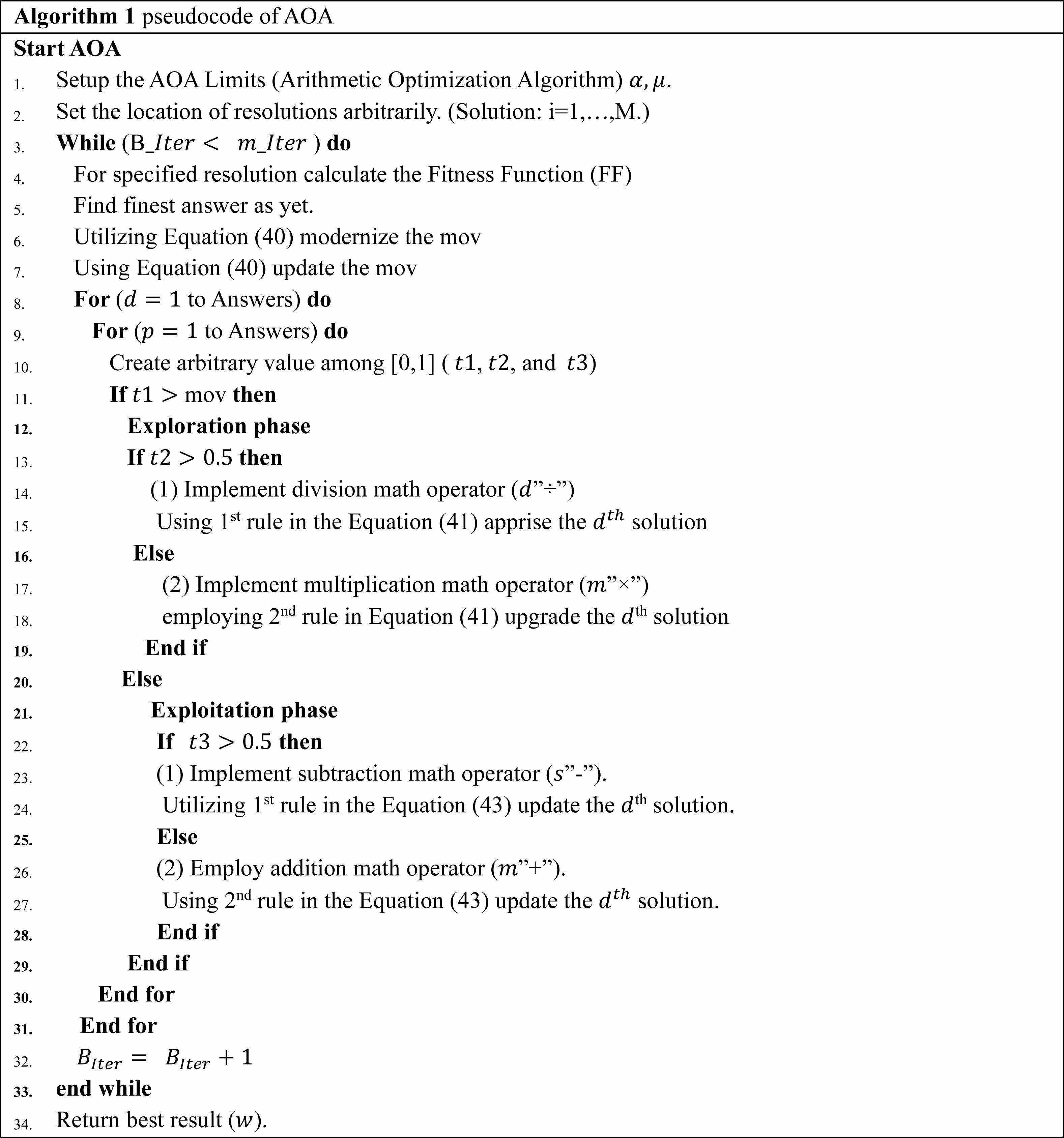
|
Fig. 1 Overall design for the proposed model. |
|
Fig. 2 Image recognition using HOG |

|
Fig. 3 Representation of a 9-bin histogram. |
|
Fig. 4 Example of technique for calculation of 9 bin histograms. |
|
Fig. 5 (a) 3×3 sample block. (b) Sign Component. |
|
Fig. 6 Two different images having same histogram. |
In this subdivision result and discussion of the suggested model is presented.
Experimental setup
The proposed model has applied Python. 70% of collected data has been used for training and 30% for testing. A comparative analysis has been made with state-of-the-art methods. The assessment considered several metrics like sensitivity, specificity, accuracy, precision, FPR, FNR, NPV, F-Measure and MCC.
Overall performance analysis for deep learning models
For Training Rate=70%
Table 1 shows the results acquired with the proposed as well as existing classifiers for 70%. The accuracy recorded by the proposed model (defectfuse classifier) is 97.4%, which is better than CNN=96.8%, Bi-LSTM =93.3%, RNN=95.6%, DCNN=93.4% due to the proposed model is the combination of CNN, Bi-LSTM, RNN. The precision is recorded by the proposed model is 88.5% which is better than CNN, Bi-LSTM, RNN, DCNN due to the involvement for ADOA. In addition, the planned model has recorded the highest sensitivity (88.5%) and specificity (98.5%) which is better than CNN, Bi-LSTM, RNN, DCNN because of the proposed model of feature selection process. The f_measure recorded by the proposed model is 88.5% which is better than remaining model due to the performance for combination of proposed model. The model recorded the high MCC of 87% than other models due to the performance of ADOA. The proposed model achives high NPV of 98.5% than other models for finding the Negative value. The model achives less FPR 1.4% and FNR 11.4% of proposed false positive and negative rate due to the involvement of deep learning technique.
For Training Rate=80%
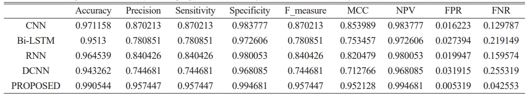
Table 2 shows the results acquired with proposed as well as existing classifiers for 80%. The defectfuse classifier, a suggested model, outperforms other models with a 99% accuracy, outperforming CNN (97.1%), Bi-lstm (95.1%), RNN (96.4%), and DCNN (94.3%). The reason for this advantage is that the suggested model integrates RNN, CNN, and Bi_LSTM. In addition, the suggested model’s precision of 95.7% beats CNN, Bi-LSTM, RNN, and DCNN since it makes use of a hybrid optimization technique. Furthermore, when contrasted to CNN, Bi-LSTM, RNN, and DCNN, the model that was suggested has the greatest sensitivity (95.7%) then specificity (99.4%). This benefit is ascribed to the property selection procedure that the proposed framework uses.The hybrid optimization approach allows the suggested model to outperform alternatives, resulting in a high MCC score of 95.2%. When it comes to recognizing negative values, the model recommended outperforms other models with a high NPV of 99.4%. The recommended model uses deep learning techniques, which lowers the FPR to 0.5% and the FNR to 4.2%. So, it is best approach for ceramic tile surface defect detection.
The superiority of the proposed defectfuse classifier over existing methods lies in its innovative design and its ability to address key challenges inherent in ceramic tile surface defect detection. Here’s a breakdown of the justification based on the results:
● Integration of Deep Learning Architectures: By combining CNN, Bi-LSTM, and RNN architectures, the proposed model harnesses the complementary strengths of these networks. CNNs excel at spatial feature extraction, Bi-LSTMs handle sequential data effectively, and RNNs capture temporal dependencies. This integration allows the model to capture intricate patterns and variations in ceramic tile images more comprehensively than single-network approaches.
● Hybrid Optimization for Feature Selection: The hybrid optimization approach, which combines arithmetic optimization algorithms and dingo optimization, ensures that the most relevant features are selected for defect detection. This optimization strategy enhances the model’s ability to discriminate between defective and non-defective tiles by focusing on the most informative features while minimizing the risk of overfitting.
● Superior Performance Metrics: The experimental results demonstrate that the proposed defectfuse classifier consistently outperforms existing classifiers across various performance metrics, including accuracy, precision, sensitivity, specificity, MCC, and NPV. These metrics serve as objective measures of the model’s effectiveness in accurately identifying defects while minimizing false positives and false negatives.
● Reduced Error Rates: Compared to existing classifiers, the proposed model exhibits lower false positive and false negative rates (FPR and FNR), indicating its ability to minimize both type I and type II errors. This reduction in error rates is crucial for ensuring that defective tiles are accurately identified and appropriate actions are taken to maintain product quality.
● Comprehensive Validation: The validation of the defectfuse classifier using a robust experimental setup, including training and testing on separate datasets, enhances the reliability and reproducibility of the results. The model’s consistent performance across different training rates further validates its effectiveness across varying data scenarios.
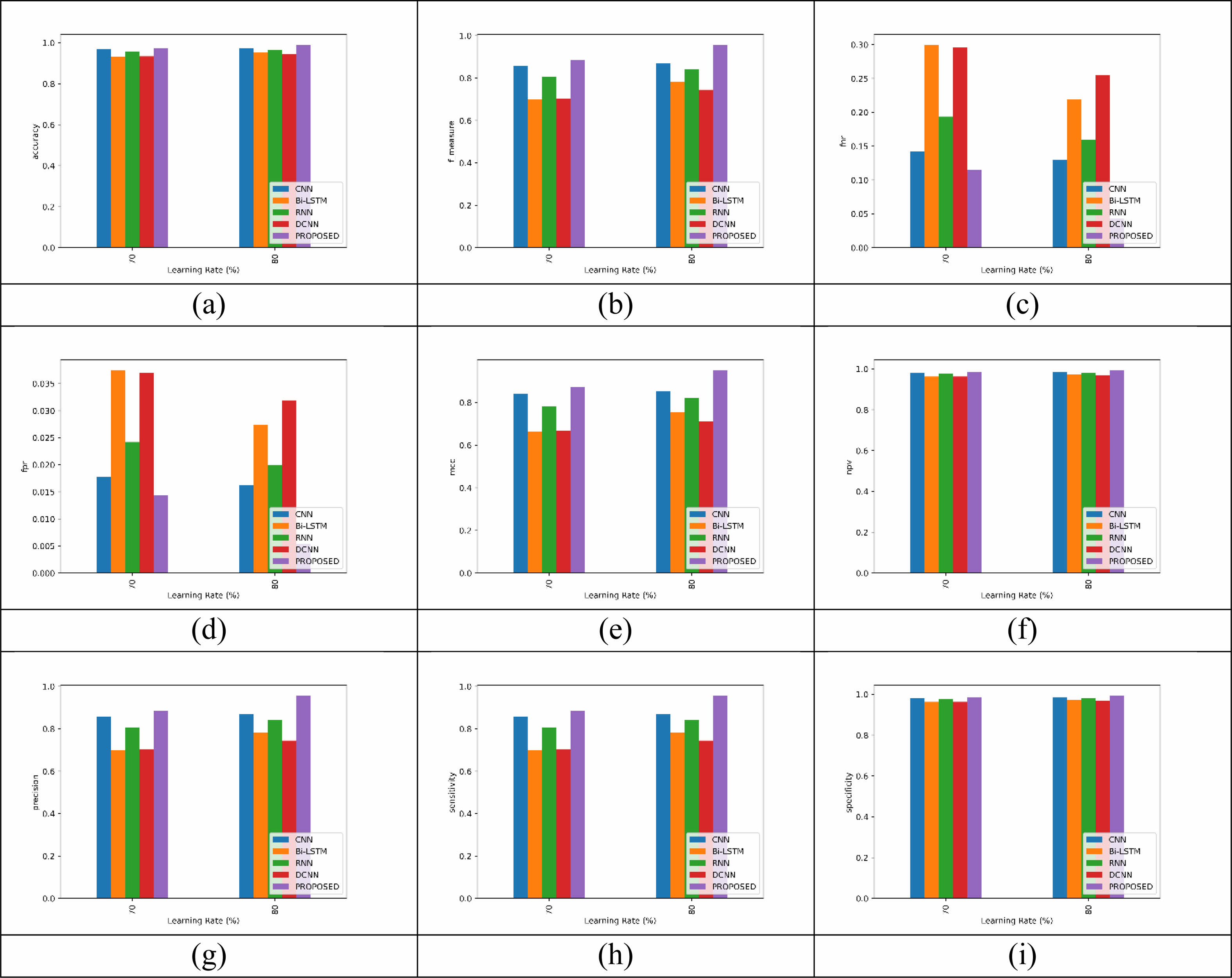
In summary, the proposed defectfuse classifier offers a holistic solution to the challenges of ceramic tile surface defect detection by leveraging advanced deep learning architectures and innovative optimization techniques. Its superior performance metrics, coupled with reduced error rates and comprehensive validation, justify its superiority over existing methods in enhancing quality control processes in the ceramic tile manufacturing industry. Fig. 7
|
Fig. 7 Classifier performance Analysis for (a) accuracy, (b) F_measure, (c) FNR, (d) FPR, (e) MCC, (f) NPV, (g) Precision, (h) Sensitivity, (i) Specificity. |
|
Table 2 Overall performance analysis for proposed Vs existing classifiers: for training rate=80% |
This research work has introduced a new deep learning approach for ceramic tile surface defect detection. (a) Data Acquisition (b) Pre-processing (c) Feature Extraction (d) Feature selection (e) Deep-learning based defect detection. Firstly, defect detection was conducted using images from the raw images of the sample. The collected images were pre-processed through median filtering and image augmentation. The processed images were endowed with features like HOG, LBP, Color Histograms, Gabor Filters, and Edge Detector. Among these features, the optimal features were determined using the new ADOA (combined arithmetic optimization algorithms and dingo optimization). Subsequently, the defect was detected with the proposed model using a new Defectfuse classifier model. The proposed Defectfuse classifier model comprised deep learning classifications such as CNN, Bi-LSTM, and RNN, respectively. Finally, the results for voting classifiers were validated. Python was used to performed in the system.
- 1. Q. Lu, J. Lin, L. Luo, Y. Zhang, and W. Zhu, Adv. Eng. Inform. 53[8] (2022) 101692.
-

- 2. Y. Sun, T. Wu, Y. Bao, Y. Li, D. Wan, K. Li, and L. He, Int. J. Appl. Ceram. Technol. 19[1] (2022) 604-611.
-
- 3. C. Wang, S. Wang, X. Li, Y. Liu, X. Zhang, Q. Chang, and Y. Wang, Int. J. Appl. Ceram. Technol. 18[3] (2021) 1052-1062.
-
- 4. G. Wan, H. Fang, D. Wang, J. Yan, and B. Xie, Ceram. Int. 48[8] (2022) 11085-11093.
-
- 5. R. Alamsyah and A.D. Wiranata, Sci. Res. J. VII[4] (2019) 41-45.
-
- 6. B. Zorić, T. Matić, and Ž. Hocenski, ISA Trans. 125[6] (2022) 400-414.
-
- 7. X. Yu, Q. Yu, Q. Mu, Z. Hu, and J. Xie, Appl. Sci. 13[21] (2023) 12057.
-
- 8. O. Stephen, U.J. Maduh, and M. Sain, Electronics 11[1] (2021) 55.
-
- 9. S. Ye and L. Sun, J. Phys.: Conf. Ser. 1650[3] (2020) 032045.
-
- 10. K.B. Kim, D.H. Song, and H.J. Park, Indones. J. Electr. Eng. Comput. Sci. 19[3] (2020) 1505-1511.
-
- 11. N.T. Huynh, D.D. Ho, and H.N. Nguyen, Sustainability 15[6] (2023) 5455.
-
- 12. Z. Zhou, Q. Lu, Z. Wang, and H. Huang, Sensors 19[22] (2019) 5000.
-
- 13. K. Wang, Z. Li, and X. Wang, Appl. Sci. 12[3] (2022) 1249.
-
- 14. M.F. Ohemu, Z.O. Zubair, and R.E. Donatus, ATBU J. Sci. Technol. Educ. 10[2] (2022) 170-180.
- 15. A. Ravendran and S. Rianmora, J. Comput. Appl. Res. Mech. Eng. 10[2] (2021) 391-404.
-
- 16. J. Wang, G. Yi, S. Zhang, and Y. Wang, Appl. Sci. 11[1] (2020) 283.
-
- 17. H.S. Nogay, T.C. Akinci, and M. Yilmaz, Neural Comput. Appl. 34[2] (2022) 1423-1432.
-
- 18. J. Wang, Z. Wu, W. Hu, C. Song, X. Guo, P. Cao, L. Yang, and Z. Zhu, Investigation on distributed rescheduling with cutting tool maintenance based on nsga-iii in large-scale panel furniture intelligent manufacturing.Journal of Manufacturing Processes, 112(Feb.) (2024) 214-224.
- 19. F. Sušac, T. Matić, I. Aleksi, and T. Keser, Bull. Pol. Acad. Sci. Tech. Sci. 69[3] (2021) e137121.
-
- 20. Oglakci, B., et al. "The Effect of Different Polishing Systems on the Surface Roughness of Nanocomposites: Contact Profilometry and SEM Analyses." Operative Dentistry 46[2] (2021) 173-187.
- 21. S. Boovaneswari, S. Nirmal, V. Meyappan, and B. Nandakumar, Semicond. Optoelectron. 42[1] (2023) 1082-1095.
- 22. W. Qian, X. Yu, W. Xie, L. Zhang, and W. Wu, J. Phys.: Conf. Ser. 2044[1] (2021) 012105.
-
- 23. X. Le, J. Mei, H. Zhang, B. Zhou, and J. Xi, Neurocomputing 408[9] (2020) 112-120.
-
- 24. G.S. Junior, J. Ferreira, C. Millán-Arias, R. Daniel, A.C. Junior, and B.J. Fernandes, Appl. Sci. 11[13] (2021) 6017.
-
- 25. H.R. Ravikumar, Y.K. Sharma, and S. Raghav, Int. J. Innov. Sci. Eng. Technol. 7[2] (2020) 252-263.
- 26. K. Avazov, M.K. Jamil, B. Muminov, A.B. Abdusalomov, and Y.I. Cho, Sensors 23[16] (2023) 7078.
-
- 27. S. Gundu and H. Syed, Sensors 23[5] (2023) 2569.
-
- 28. P. Banerjee, A.K. Bhunia, A. Bhattacharyya, P.P. Roy, and S. Murala, Expert Syst. Appl. 113[12] (2018) 100-115.
-
- 29. F. Bianconi, A. Fernández, F. Smeraldi, and G. Pascoletti, J. Imaging 7[11] (2021) 245.
-
- 30. H. Kim, Y. Arisato, and J. Inoue, Unsupervised segmentation of microstructural images of steel using data mining methods. Computational Materials Science. 201[5] (2022) 110855.
-
- 31. G. Lambard, K. Yamazaki, and M. Demura, Generation of highly realistic microstructural images of alloys from limited data with a style-based generative adversarial network. Scientific Reports 13[1] (2023) 566.
- 32. L. Abualigah, A. Diabat, S. Mirjalili, M. Abd Elaziz, and A.H. Gandomi, Comput. Methods Appl. Mech. Eng. 376[4] (2021) 113609.
-
- 33. D. Bhatt, C. Patel, H. Talsania, J. Patel, R. Vaghela, S. Pandya, K. Modi, and H. Ghayvat, Electronics 10[20] (2021) 2470.
-
- 34. E. Cumbajin, N. Rodrigues, P. Costa, R. Miragaia, L. Frazão, N. Costa, A. Fernández-Caballero, J. Carneiro, L.H. Buruberri, and A. Pereira, J. Imaging 9[10] (2023) 193.
-
 This Article
-
2024; 25(4): 572-588
Published on Aug 31, 2024
- 10.36410/jcpr.2024.25.4.572
- Received on Mar 8, 2024
- Revised on Apr 26, 2024
- Accepted on Apr 29, 2024
Services
- Abstract
introduction
literature review
proposed methodology
result and discussion
conclusion
- References
- Full Text PDF
Shared
Correspondence to
- Chi Zhang
-
Liaocheng Vocational and Technical College, Liaocheng, Shandong, 252000, China
Tel : 0635-8334969 Fax: 8322030 - E-mail: zhangchi292@163.com
Clean-Energy Research Institute(CRI), Hanyang University, 222, Wangsimni-ro, Seongdong-gu, Seoul, 04763, Korea
E-mail: jcpr@hanyang.ac.kr